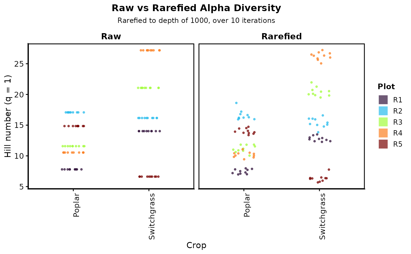
Variance propagation diagnostic for rarefaction

This function evaluate the variance between rarefaction iterations from multi_rarefy() by visually comparing raw vs. rarefied alpha diversity metrics calculated at each iterations. It is possible to plot observed richness (q=0), Shannon diversity (q=1), or Simpson diversity (q=2) by setting the q parameter to "richness" or q = 0, "shannon" or q = 1, or "shannon" or q = 2. The plot is faceted by method (raw vs rarefied) and colored by a specified grouping variable from the sample data.

Usage

plot_variance_propagation(
  physeq_obj,
  rarefied,
  q = 0,
  group_var,
  group_color,
  convert_to_factor = FALSE
)

Arguments

physeq_obj

Raw phyloseq object

rarefied

Output from multi_rarefy(). Either a list of dataframes or and array.

q

Hill number order (q = 0 for richness, q = 1 for Shannon, q = 2 for Simpson)

group_var

A grouping variable to use gor grouping as in the sample_data()

group_color

A color variable to use present in the sample_data()

convert_to_factor

Logical. If TRUE, both group_var and group_color are coerced to factor before plotting, which is useful when those columns are numeric/continuous (e.g. dates, counts) but should be treated as discrete groups. When TRUE a discrete color scale (scale_color_viridis_d) is used; otherwise the continuous scale (scale_color_viridis_c) is used. Default FALSE.

Value

ggplot object comparing raw vs rarefied diversity distributions across iterations.

Examples

library(phyloseq)
library(BRCore)
# Example comparing hill q=1 between Poplar and Switchgrass plots
bcse_filt <- bcse |>
subset_samples(Crop %in% c("Poplar", "Switchgrass"))

bcse_rarefied_otutable_filt <-
 multi_rarefy(
       physeq_obj = bcse_filt,
       depth_level = 1000,
       num_iter = 10,
       .as = "list",
       set_seed = 7643
   )
#> 
#> ── Rarefaction iterations starting... ──────────────────────────────────────────
#> 
#> ── Input Validation ──
#> 
#> ✔ Input phyloseq object is valid!
#> ℹ Seed: 7643
#> ℹ Input (matrix/df dim): 10 samples x 2861 taxa
#> ℹ Rarefaction depth: 1000
#> ℹ Iterations: 10
#> ℹ taxa_are_rows: TRUE
#> ℹ OTU matrix/df rownames head: bcse73, bcse102, bcse104, bcse77, bcse78, bcse75
#> ℹ OTU matrix/df colnames head: OTU_427, OTU_11, OTU_253, OTU_148, OTU_3, OTU_78
#> ℹ Row sums summary: Min=3146, Max=67815, Median=8685.5
#> 
#> ── Rarefaction Results ──
#> 
#> ── Sample Removal 
#> ✔ No samples removed.
#> 
#> ── Taxa Removal 
#> ✔ No taxa removed.
#> ! Taxa are not removed across iterations to maintain consistent dimensions. 
#> Downstream analyses should handle zero-abundance taxa appropriately.
#> 
#> ── Data Sparsity 
#> ℹ Returning list of data frames for each iteration.
#> • Rarefied matrix (across 10 iterations):
#>   • Min: 27998 zeros (97.86% sparsity) out of 28610 entries
#>   • Max: 28029 zeros (97.97% sparsity) out of 28610 entries
#>   • Avg: 28011.6 zeros (97.91% sparsity) out of 28610 entries
#> 
#> ── Final Data Dimensions 
#> ✔ Output: 10 iterations with 10 unique samples
#> • Samples per iteration:
#>   • Min: 10
#>   • Max: 10
#> • Non-zero taxa per iteration:
#>   • Min: 188
#>   • Max: 200
#>   • Avg: 193.1

plot_variance_propagation(
   physeq_obj   = bcse_filt,
   rarefied = bcse_rarefied_otutable_filt,
   q        = 1,
   group_var = "Crop",
   group_color = "Plot"
)
#> ✔ Input phyloseq object is valid!
#> 
#> ── Rarefaction Variance Propagation Visualization ──────────────────────────────
#> ℹ Hill number order selected, q= 1
#> ℹ Number of rarefaction iterations, n_iter= 10
#> ℹ Comparison plot generated!